In the mid-1980s, the mathematician Yves Mayer from the University of Marseille and the petroleum engineer Jaean Morlet participated in the work of analyzing data from petroleum surveys for Elf-Aquitaine. In their quest to find a better method, they rediscovered a set of a new type of transforms they called Wavelets. The wavelet transform solved some of the weaknesses of the Fourier transform from Fourier. The method required less computing power and it was possible to identify period and phase relationships in time series. When the method was presented, Morlet received the comment: “A method, which is not described in a textbook, cannot be of great importance”. In 1988, Ingrid Daubechies published the article “Orthogonal Bases of Compactly Supported Wavelets”. This was perhaps the most important method of analyzing time series since Fourier published his method in 1822.
I started using wavelet spectrum analysis approx. year 2000. The problem was to find coincidences between changes in the ecosystem and temperature variations in the Barents Sea. Wavelet transforms have many variants that give different results. This made it necessary to examine most of the available wavelet transforms in the MATLAB Toolbox.
When I submitted my first manuscript for review, wavelet spectrum analysis was unknown to the editor. To find a reviewer, I visited the EGU conference in Vienna. Here I found two young PhD students studying the wavelet transform. Gradually, more people began to use the wavelet transform to study climate time series. Still, most scientists use the wavelet transform as a substitute for Fourier analysis. To me, this is the wrong use of this powerful method.
Wavelet transform
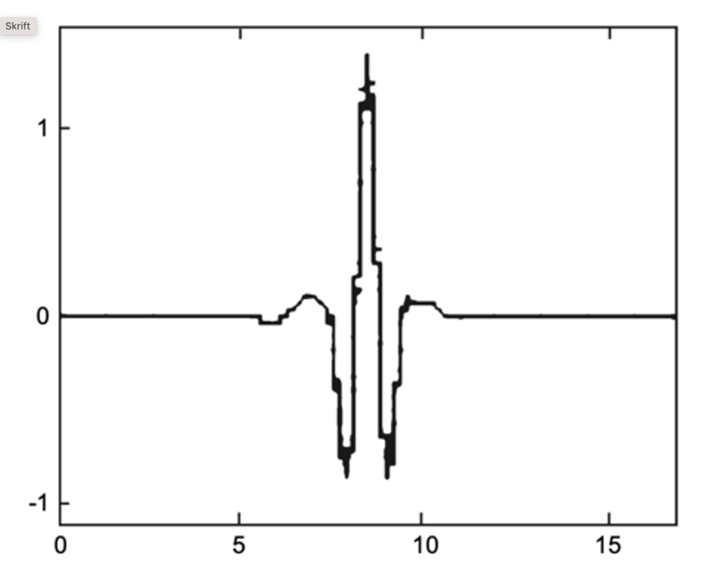
Figure 1 Wavelet pulse function h(t).
A Fourier transform is based on correlation between a time series x(t) and a set of sine functions sin(2p/T). A wavelet transform is based on a moving correlation between a time series x(t) and an impulse function h(t) (Figure 1). The correlated wave function s(t) will respond when there is a match between x(t) variations and the pulse function h(t). Longer pulse periods will have a correlation to longer periods in x(t). A set of wavelet pulses calculates a wavelet spectrum for all pulse variations in the time series x(t). Each wavelet reveals the position of a pulse variation in the time series x(t). The maxima and minima of the pulse position reveal the phase of the period. Information about phase is needed to have a complete time series signature S(T, F(t-t0)), where t0 represents the time when a cycle period T has a maximum.
Example 1. Identify two sine functions.
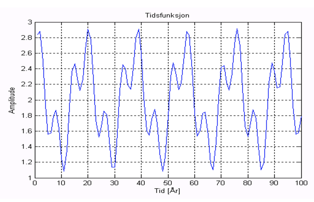
Figure 2 Sum of two sinus periods.
A time series is produces by the simple model:
x(t) = 1.9 +0.4sin(2pi/T1 + F1) + 0.6sin(2pi/T2 + F2)
where the cycle period T1 = 18.6/3 = 6.2 years, the phase angle F1= -0.29(rad), T2 = 18.6 years, and F2 = 1.52(rad). The question is how a wavelet spectrum analysis can help us to identify time series signature S(T, F(t-t0)).
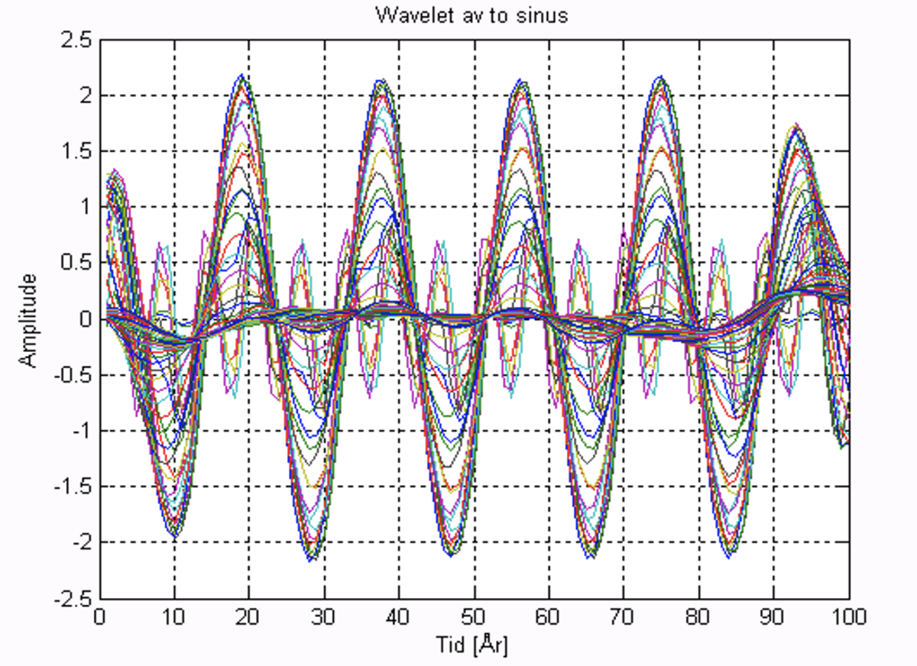
Figure 3. Computed wavelet spectrum
The first thing we should do is subtract the mean by setting x(t) = x(t)-E[x(t)]. This avoids spurious periods at the ends of the time series. The next step is to normalize the time series by dividing the variance.
Figure 3 shows the calculated wavelet spectrum of the time series x(t), where the x-axis represents the development over time and the y-axis represents moving correlation between x(t) and a scalable feature h(t). The Y-axis has a maximum when the pulse width h(t) coincides with the period times T1 and T2. The time of maximum correlation reveals the phase of periods T1 and T2.
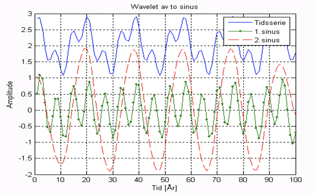
Figure 4. Time series x(t) and identified periods in the wavelet spectrum
Figure 4 shows the time series, x(t), and identified periods of approximately T1 = 6 years and T2. = 18 in the wavelet spectrum. The cycle periods are identified by calculating the autocorrelation of the wavelet spectrum. The cycle period phase has maxima and minima in the wavelet spectrum. It appears from the figure that the wavelet spectrum has revealed the x(t) signature S(T, F(t-t0)), where T = [6, 18] and F(t0) = [39, 39 ].
Example 2. Total solar irradiation
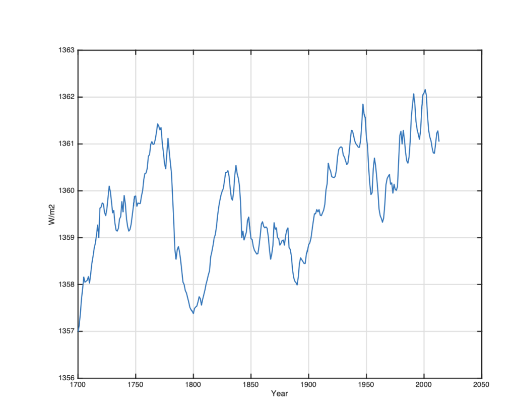
Figure 5. Total solar irradiance from the years 1700 to 2013 (Scafetta & Willson, 2014).
Total solar irradiation (TSI) represents the measured irradiance Wm-2 at the average distance from the sun to the earth. Figure 5 shows an annual average time series for total solar radiation covering the period from 1700 to 2013 (Scafetta & Willson, 2014). A simple visual inspection of this time series shows that TSI from the sun has variations, and TSI has an average growth from 1700 to 2014. The research question is to uncover the source of TSI variations.
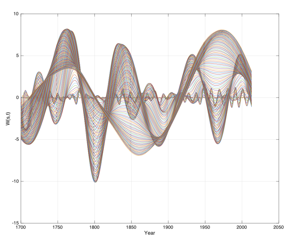
Figure 6. Calculated wavelet spectrum W(s, t) of the TSI data series (Figure 5) (Yndestad and Solheim 2017).
The transformed wavelet spectrum Whs(s, t) (Figure 6) represents a set of separated wavelet periods from the TSI data series from 1700 to 2013. In this presentation, the wavelet scaling range is s = 1 . . . 0.5N, and the data series contains N = (2013-1700) = 313 data points. A visual inspection of the TSI wavelet spectrum shows dominant periods in the TSI data series in the years between 1700 and 2013. The long wavelet period has a maximum in 1760, 1840, 1930 and 2000, with an average time difference of approx. 80 years.
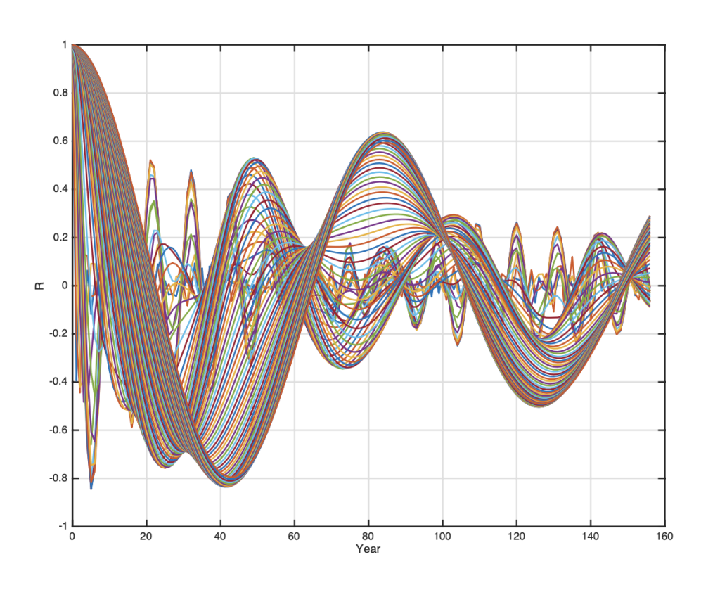
Figure 7. Autocorrelations R(m) of the TSI wavelet spectrum (Figure 6) (Yndestad and Solheim 2017).
The autocorrelation of the wavelet spectrum W(s, t), is calculated as R(m) = E[W(s, t)W(s, (t+m)], is shown in Figure 7. (Yndestad and Solheim 2017). Calculated signature spectrum revealed for the first time that the Jovian planets are the source of TSI variations. The result was confirmed by the signature of the Sun’s motion around the Sun’s Barycenter A study of Jovian planetary motions has revealed a direct link between Jovian planetary motion, solar position motion and TSI -variations in periods up to 4450 years (Yndestad 2022).
Wavelets in climate science
The wavelet spectrum paradigm calculates periods and period phase relationships in a time series x(t). When the periods and phase are known, we can:
- calculate phase delay between time series.
- calculate period and phase relationships in a chain of events.
- can calculate interference between a period’s maximum and minimum.
- calculate extreme climate maxima and deep minima.
- calculate future maxima and minima in upcoming events.
It has been possible to calculate periodic events, from the oscillating solar system to the oscillating motion of the Earth’s axis, tidal fluctuations, lunar forced climate periods, solar forced climate periods, marine ecosystem oscillations and much more. The difference between deterministic astronomical periods and estimated wave periods in climate data series is only 0-5 years.
Key papers
- Yndestad H. (2006). The influence of the lunar nodal cycle on Arctic climate. ICES Journal.
- Yndestad Harald; William R. Turrell; Ozhigin Vlatimir. (2008). Lunar nodal tide effects on variability of sea level, temperature, and salinity in the Faroe-Shetland Channel and the Barents Sea. Deep-Sea Research I.
- Yndestad H. (2009). The influence of long tides on ecosystem dynamics in the Barents Sea. Deep-Sea Research II.
- Yndestad Harald; Solheim Jan-Erik. (2016). The Influence of Solar System Oscillation on the Variability of the Total Solar Irradiance. New Astronimy
- Yndestad H. 2022. Jovian Planets and Lunar Nodal Cycles in the Earth’s Climate Variability Frontiers in Astronomy and Space Sciences. May 10. 2022. https://doi.org/10.3389/fspas.2022.839794

Greetings! Very useful advice in this particular post!
It’s the little changes which will make the most important changes.
Thanks for sharing!